Beer: A ‘Case’ Study

A Case Study of US Craft Beer and Breweries

Introduction and Overview

This case study explores datasets for various beers and breweries where they are produced in the US. The steps and procedures taken for this analysis are detailed below.

The initial data provided were in two separate datasets, one each for beers and the other breweries. The dataset combined into a single dataset using Full join.

Repository Structure

For Repository files, please see our Github

ReadMe.md: This is the base page for the repository, containing an introduction as well as our codebook for how we coded variable names throughout the datasets.
BeerCaseStudy.Rmd : This is the primary file for the analysis, and is the file we are currently reading. It contains all the relevant R code, graphics, and analysis for the project; also included are specific .docx, .html, and .pdf knitted versions of this file.
Beers.csv and Breweries.csv, were provided and are the original datasets from which our merged dataset is produced.

Reproduction of Analysis

README.md is the suggested place to start. It is also the possible method to downlaod this repository.

We begin by setting knitr options,

# Read in beer and breweries data set using _csv for more tidy output
Beers <- read_csv('./data/Beers.csv', col_types = cols())
Breweries <- read_csv('./data/Breweries.csv', col_types = cols())

Research Questions

1. How many breweries are present in each state?

We can answer this question by counting the number of values of each State from the Breweries dataset.

# Format for output:
BPS <- data.frame(table(Breweries$State))
colnames(BPS) <- c('State','Breweries')
BrewPerState <- cbind(BPS[1:11,], BPS[12:22,], BPS[23:33,], BPS[34:44,], BPS[45:55,])

# Stylized output:
kable(BrewPerState, caption = 'Breweries per State') %>% kable_styling()

Breweries per State
State	Breweries	State	Breweries	State	Breweries	State	Breweries	State	Breweries
AK	7	HI	4	MI	32	NV	2	UT	4
AL	3	IA	5	MN	12	NY	16	VA	16
AR	2	ID	5	MO	9	OH	15	VT	10
AZ	11	IL	18	MS	2	OK	6	WA	23
CA	39	IN	22	MT	9	OR	29	WI	20
CO	47	KS	3	NC	19	PA	25	WV	1
CT	8	KY	4	ND	1	RI	5	WY	4
DC	1	LA	5	NE	5	SC	4
DE	2	MA	23	NH	3	SD	1
FL	15	MD	7	NJ	3	TN	3
GA	7	ME	9	NM	4	TX	28

# Set up the map:
Breweries <- rename(Breweries, state = State)
map <- Breweries %>% group_by(state) %>% summarise(Breweries = n())

# Plot Brewery heatmap:
plot_usmap(data=map, values = "Breweries", labels=F) + 
  labs(title = "Breweries per State") +
  scale_fill_continuous(name = "Breweries")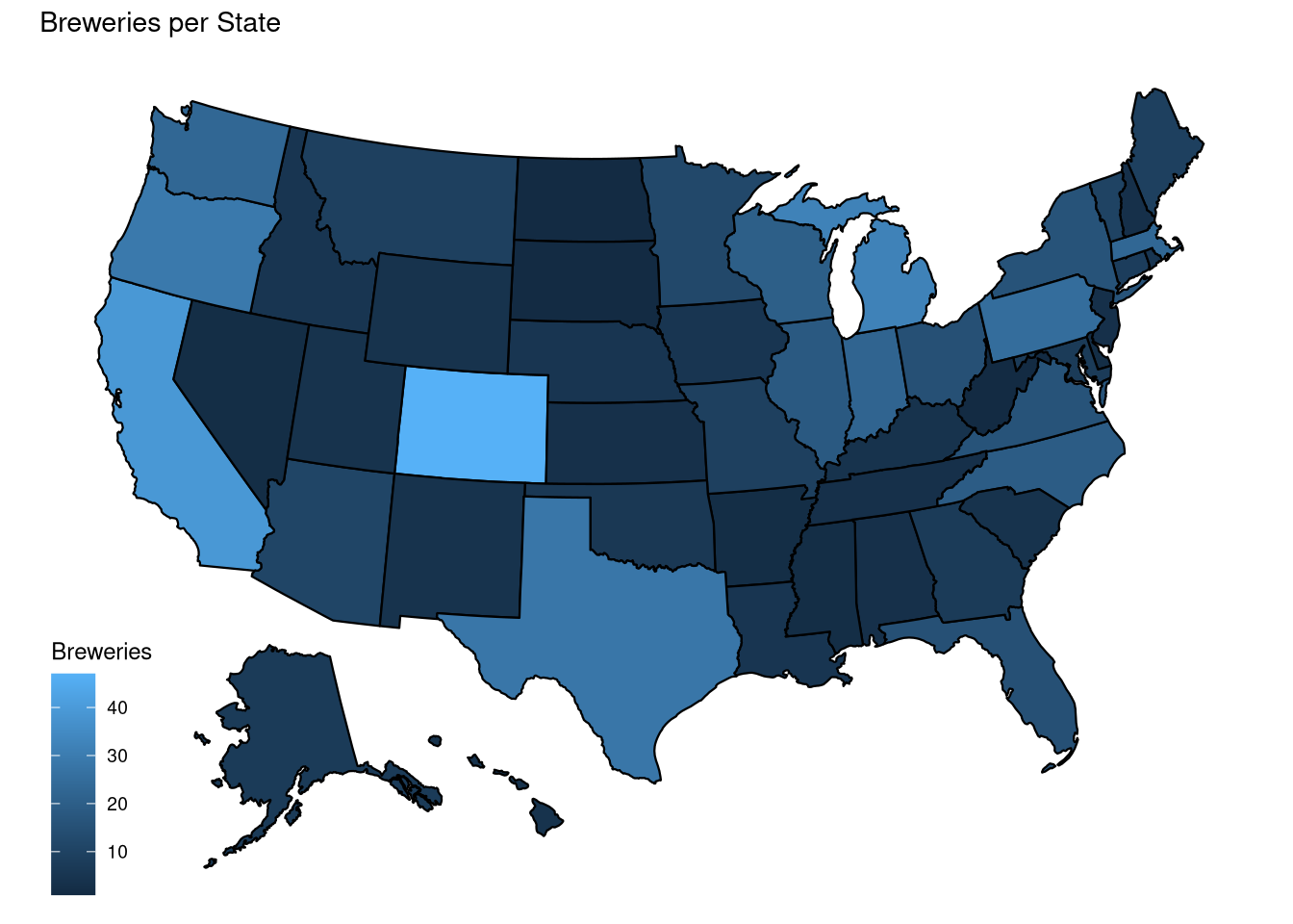

2a. Merge beer data with the breweries data.

The field Brewery_id in Beers.csv and Brew_ID in Breweries.csv share the same data, but do not share a name. We remedy this by renaming the column in Beers.csv.

After renaming, we can merge them into a single dataset, using full_join.

# Rename Brewery_id to Brew_ID to satisfy merging requirement
Beers <- rename(Beers, Brew_ID = Brewery_id)

# Merge tables
Brewdata <- full_join(Beers, Breweries, by="Brew_ID")

# Change variable names to more meaningful title
Brewdata <- rename(Brewdata, Beer = Name.x, Brewery = Name.y, OZ = Ounces)

#Convert OZ to factor
Brewdata$OZ = as.factor(Brewdata$OZ)

beer <- Brewdata %>% filter(!is.na(IBU) & !is.na(ABV) & !is.na(Style))
ggplot(beer, aes(x=state, y=ABV)) + geom_boxplot(fill= "#75AADB")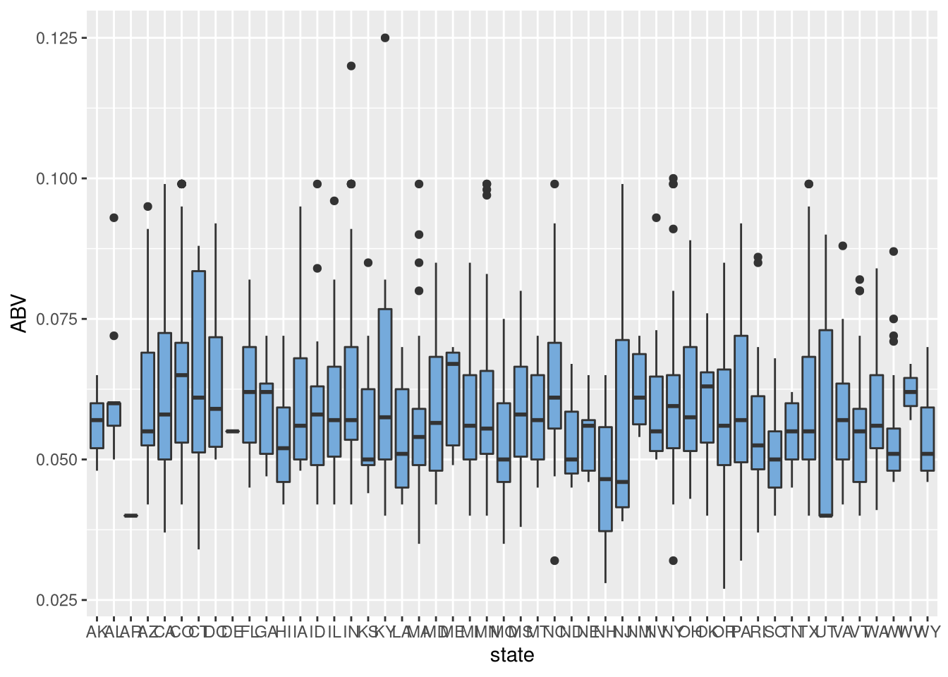

write.csv(beer, "beer.csv")


beer %>% filter(state %in% c('AZ'))

## # A tibble: 23 x 10
##    Beer        Beer_ID   ABV   IBU Brew_ID Style    OZ    Brewery    City  state
##    <chr>         <dbl> <dbl> <dbl>   <dbl> <chr>    <fct> <chr>      <chr> <chr>
##  1 Barrio Bla…    2005 0.06     60     252 America… 12    Barrio Br… Tucs… AZ   
##  2 Noche Dulce    2062 0.071    16     232 America… 16    Borderlan… Tucs… AZ   
##  3 Sunbru Köl…    2309 0.052    17     161 Kölsch   12    Four Peak… Tempe AZ   
##  4 Four Peaks…    1585 0.042     9     161 Fruit /… 12    Four Peak… Tempe AZ   
##  5 Hop Knot I…     358 0.067    47     161 America… 12    Four Peak… Tempe AZ   
##  6 Kilt Lifte…     179 0.06     21     161 Scottis… 12    Four Peak… Tempe AZ   
##  7 Lumberyard…    1153 0.053    20     159 America… 12    Lumberyar… Flag… AZ   
##  8 Camelback      2312 0.061    60     158 America… 12    Phoenix A… Phoe… AZ   
##  9 Sex Panther    2599 0.069    20      31 America… 12    SanTan Br… Chan… AZ   
## 10 Winter War…    2073 0.095    25      31 Winter … 16    SanTan Br… Chan… AZ   
## # … with 13 more rows

2b. Check the first and last 6 observations to verify the merged file.

To retrieve the first and last six observations from the combined data, we run head and tail on Brewdata, our combined dataset.

kable(Brewdata %>% head()) %>% kable_styling()

Beer	Beer_ID	ABV	Brew_ID	Style	OZ	Brewery	City	state
Pub Beer	1436	0.050	409	American Pale Lager	12	10 Barrel Brewing Company	Bend	OR
Devil’s Cup	2265	0.066	178	American Pale Ale (APA)	12	18th Street Brewery	Gary	IN
Rise of the Phoenix	2264	0.071	178	American IPA	12	18th Street Brewery	Gary	IN
Sinister	2263	0.090	178	American Double / Imperial IPA	12	18th Street Brewery	Gary	IN
Sex and Candy	2262	0.075	178	American IPA	12	18th Street Brewery	Gary	IN
Black Exodus	2261	0.077	178	Oatmeal Stout	12	18th Street Brewery	Gary	IN

kable(Brewdata %>% tail()) %>% kable_styling()

Beer	Beer_ID	ABV	IBU	Brew_ID	Style	OZ	Brewery	City	state
Rocky Mountain Oyster Stout	1035	0.075		425	American Stout	12	Wynkoop Brewing Company	Denver	CO
Belgorado	928	0.067	45	425	Belgian IPA	12	Wynkoop Brewing Company	Denver	CO
Rail Yard Ale	807	0.052		425	American Amber / Red Ale	12	Wynkoop Brewing Company	Denver	CO
B3K Black Lager	620	0.055		425	Schwarzbier	12	Wynkoop Brewing Company	Denver	CO
Silverback Pale Ale	145	0.055	40	425	American Pale Ale (APA)	12	Wynkoop Brewing Company	Denver	CO
Rail Yard Ale (2009)	84	0.052		425	American Amber / Red Ale	12	Wynkoop Brewing Company	Denver	CO

3. Address the missing values in each column.

To start, we first use a function (which returns true if a given value is NA, false otherwise, using is.na) and sapply to determine the number of missing values for each column within Brewdata. This gives us a raw data view of the missing data. We then plot the missing data to visualize the quantity.

# Explore missing values with kable library to make document more presentable:
MissingValues <- sapply(Brewdata, function(x)sum(is.na(x)))
MissingValues %>% kable("html") %>% kable_styling()

	x
Beer	0
Beer_ID	0
ABV	62
IBU	1005
Brew_ID	0
Style	5
OZ	0
Brewery	0
City	0
state	0

# Missing values code borrowed from: https://jenslaufer.com/data/analysis/visualize_missing_values_with_ggplot.html

missing.values <- Brewdata %>% gather(key = "key", value = "val") %>%
  mutate(isna = is.na(val)) %>%   group_by(key) %>%
  mutate(total = n()) %>%   group_by(key, total, isna) %>%
  summarise(num.isna = n()) %>%   mutate(pct = num.isna / total * 100)


levels <- (missing.values  %>% filter(isna == T) %>% arrange(desc(pct)))$key

percentage.plot <- missing.values %>% ggplot() + geom_bar(aes(x = reorder(key, desc(pct)), y = pct, fill=isna), 
                          stat = 'identity', alpha=0.8) + scale_x_discrete(limits = levels) + 
  scale_fill_manual(name = "", values = c('steelblue', 'tomato3'), labels = c("Present", "Missing")) + 
  coord_flip() + labs(title = "Percentage of missing values", x = 'Columns with missing data', y = "Percentage of missing values")

percentage.plot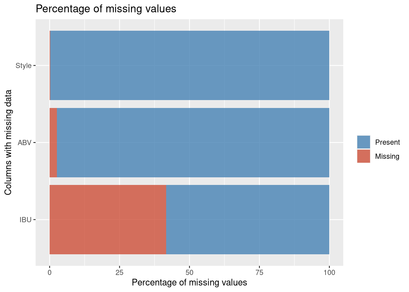

To tackle the low hanging fruit, we will remove 5 observations with missing styles, and mark the missing IBU/ABV values to compare later.
> 3/5 of these also have missing ABV and IBU values also.
> The ABV/IBU of the non-missings values aren’t remarkable, so their removal shouldn’t affect the overall data, but it is worth noting.

# remove the 5 beers missing style (3 of them were missing ABV/IBU also)
Brewdata %>% filter(is.na(Style))

## # A tibble: 5 x 10
##   Beer        Beer_ID    ABV   IBU Brew_ID Style OZ    Brewery      City   state
##   <chr>         <dbl>  <dbl> <dbl>   <dbl> <chr> <fct> <chr>        <chr>  <chr>
## 1 Special Re…    2210 NA        NA      30 <NA>  16    Cedar Creek… Seven… TX   
## 2 Kilt Lifte…    1635  0.06     21     161 <NA>  12    Four Peaks … Tempe  AZ   
## 3 OktoberFie…    2527  0.053    27      67 <NA>  12    Freetail Br… San A… TX   
## 4 The CROWLE…    1796 NA        NA     167 <NA>  32    Oskar Blues… Longm… CO   
## 5 CAN'D AID …    1790 NA        NA     167 <NA>  12    Oskar Blues… Longm… CO

RemovedBrews <- Brewdata %>% filter(is.na(Style))
Brewdata <- Brewdata %>% filter(!is.na(Style))

# identify missing IBU/ABV values:
Brewdata$ImputedABV <- ifelse(is.na(Brewdata$ABV),'Imputed','Original')
Brewdata$ImputedIBU <- ifelse(is.na(Brewdata$IBU),'Imputed','Original')

Now that we’ve marked the missing values, we can explore imputation of 62 missing ABV and 1005 missing IBU values into BrewComplete (so we can compare vs Brewdata).

# view random sample of imputed vs original plot ABV:
set.seed(10)
StyleSample <- sample(unique(BrewComplete$Style), size=15)

BrewComplete %>% filter(Style %in% StyleSample) %>% ggplot(aes(x=ABV, y=reorder(Style,ABV), color=ImputedABV)) + geom_point() + labs(y = 'Style')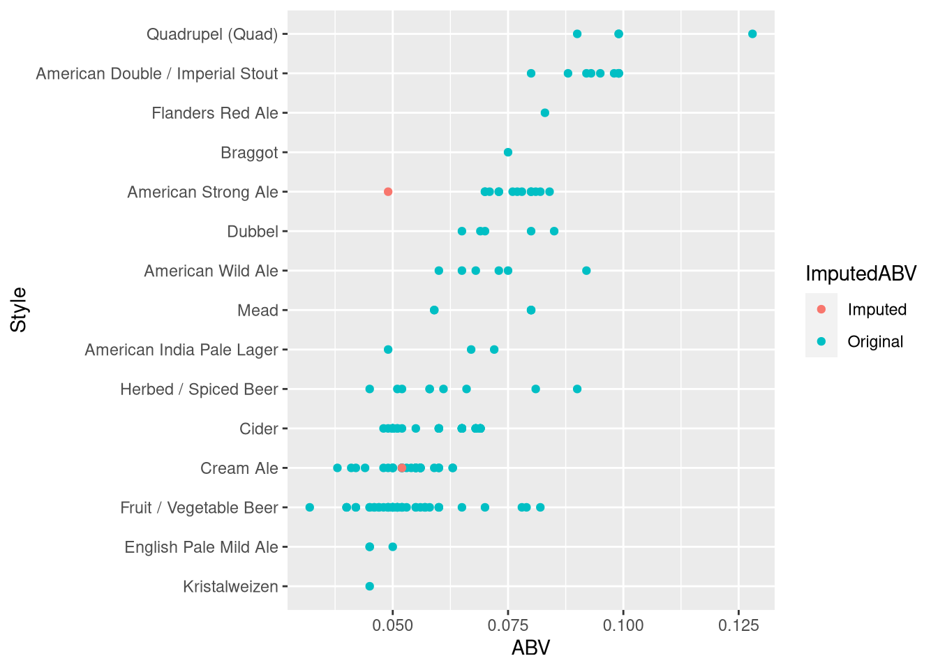

# view random sample of imputed vs original plot IBU:
BrewComplete %>% filter(Style %in% StyleSample) %>% ggplot(aes(x=IBU, y=reorder(Style,IBU), color=ImputedIBU)) + geom_point() + labs(y = 'Style')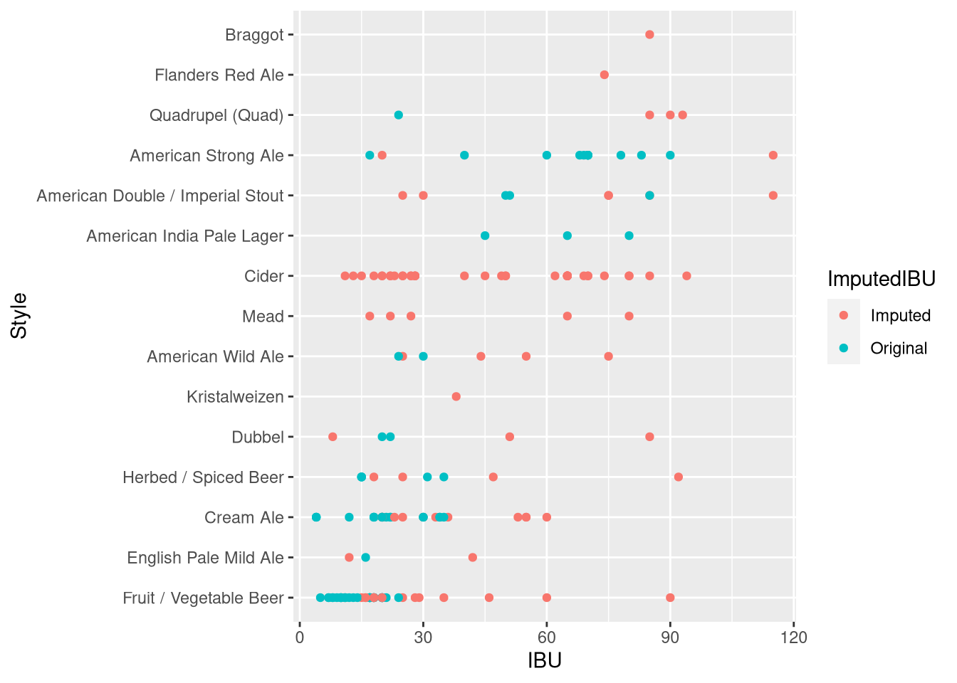

# assign imputed ABV values
Brewdata$ABV <- BrewComplete$ABV

# store IBU containing dataset for further examination 
IBUdata <- Brewdata %>% filter(!is.na(IBU))

Based on visual inspection, it appears ABV is safe to impute, but IBU looks like it might be overreaching! (e.g. Cider Beer IBUs have no reference data for comparison)

We will exclude beer data with missing IBU for comparisons using IBU in future tests.

4. Compare the median alcohol content and international bitterness unit for each state.

Arkansas and Utah are tied for lowest ABV at 4.0% Maine has highest ABV at 6.7%

Wisconsin has the lowest IBU @ 19 Maine has the highest IBU @ 61

# 4.a transform the data
Firewater <- Brewdata %>% na.omit() %>% group_by(state) %>% summarise(Median = median(ABV)) %>% arrange(Median)
Bitter <- Brewdata %>% na.omit() %>% group_by(state) %>% summarise(Median = median(IBU)) %>%  arrange(Median)

# 4.b Plot a bar chart to compare ABV by state
ggplot(data=Firewater, aes(x=state, y=Median)) +
  geom_bar(stat="identity", fill="steelblue")+
  theme_economist() + 
  scale_color_economist()+
  theme(axis.text.x=element_text(size=rel(0.8), angle=90)) +
  ggtitle("Median ABV by State") +
  labs(x="state",y="ABV")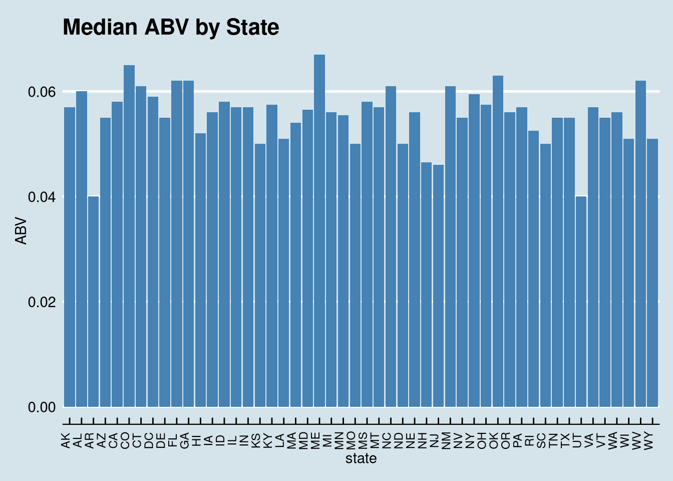

# 4.c Plot a bar chart to compare IBU by state
ggplot(data=Bitter, aes(x=state, y=Median)) +
  geom_bar(stat="identity", fill="steelblue")+
  theme_economist() + 
  scale_color_economist()+
  theme(axis.text.x=element_text(size=rel(0.8), angle=90))+
  ggtitle("Median IBU by State") +
  labs(x="State",y="IBU")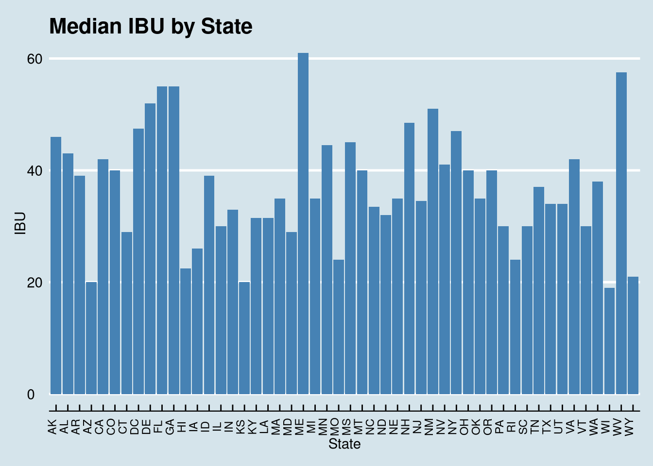

# Combined plot merging 4b and 4c:
Brewdata %>% filter(!is.na(IBU & ABV)) %>% select(state, ABV,IBU) %>%
  group_by(state) %>%
  dplyr::summarize(Median_IBU=median(IBU), Median_ABV=median(ABV*100)) %>%
  gather(`Median_IBU`, `Median_ABV`, key='Type', value='Measurement') %>%
  ggplot(aes(state, Measurement, fill=Type)) +
  geom_bar(stat='identity', position = 'Dodge') +
  labs(y='ABV% and IBU', title = 'Median ABV and IBU by State') +
  theme_economist() + 
  scale_fill_manual(name = "", values = c('tomato3','steelblue'), labels = c("ABV %", "IBU")) +
  scale_color_economist() +
  theme(axis.text.x=element_text(size=rel(0.8), angle=90))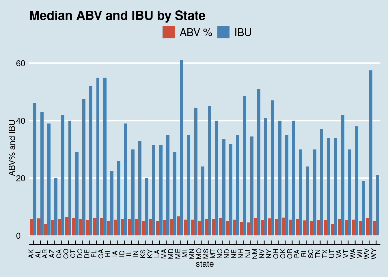

5. Which state has the maximum alcoholic (ABV) beer? Which state has the most bitter (IBU) beer?

We identify Colorado as having the beer with the highest ABV, at .128; and we identify Oregon has having the beer with the highest IBU, at 138.

TopABV <- top_n(Brewdata, 1, ABV)
TopIBU <- top_n(Brewdata, 1, IBU)
kable(TopABV) %>% kable_styling()

Beer	Beer_ID	ABV	IBU	Brew_ID	Style	OZ	Brewery	City	state	ImputedABV	ImputedIBU
Lee Hill Series Vol. 5 - Belgian Style Quadrupel Ale	2565	0.128		52	Quadrupel (Quad)	19.2	Upslope Brewing Company	Boulder	CO	Original	Imputed

kable(TopIBU) %>% kable_styling()

Beer	Beer_ID	ABV	IBU	Brew_ID	Style	OZ	Brewery	City	state	ImputedABV	ImputedIBU
Bitter Bitch Imperial IPA	980	0.082	138	375	American Double / Imperial IPA	12	Astoria Brewing Company	Astoria	OR	Original	Original

# Set up the map:
df <- data.frame(abbr=c('CO','OR'),Top_Beer=c('ABV','IBU'))
map <- left_join(statepop,df, by ='abbr')

# Plot the map:
plot_usmap(data = map, values = "Top_Beer") + labs(x='',y='',title = "Top States by ABV/IBU") +
  scale_discrete_manual(labels(remove)) + scale_fill_manual(name = "Category", values=c(ABV='tomato3',IBU='steelblue'), na.value='darkgrey') + theme(legend.background = element_rect(fill = "#D5E4EB"), plot.background = element_rect(fill = "#D5E4EB"))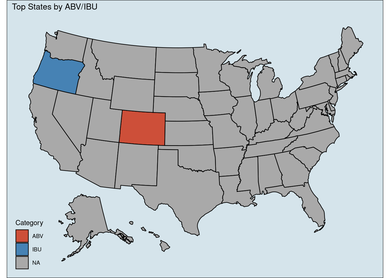

6. Comments on the summary statistics and distribution of the ABV variable.

We get summary statistics by calling summary and sd on the ABV column in our Brewdata dataset.

The ABV of all measured beer falls into a range of .1% to 12.8% alcohol content by volume. The data appears to be fairly normally distributed with a touch of right skewness, with a mean of 5.97%, a median of 5.60%, a standard deviation of 1.35% and an interquartile range of 1.7%.

summary(Brewdata$ABV)

##    Min. 1st Qu.  Median    Mean 3rd Qu.    Max. 
## 0.00100 0.05000 0.05600 0.05975 0.06700 0.12800

sd(Brewdata$ABV)

## [1] 0.01348271

# Plot the histogram:
Brewdata %>% ggplot(aes(ABV)) + 
  geom_histogram(binwidth = .01, fill='steelblue', color='black') + 
  theme_economist() + 
  labs(y='Count of Beers', title='ABV Summary')

ABV of all measured beer falls into a range of .1% to 12.8% alcohol content by volume. The data appears to be fairly normally distributed with a touch of right skewness, with a mean of 5.97%, a median of 5.60%, a standard deviation of 1.35% and an interquartile range of 1.7%.

Median ABV = 5.6%
Mean ABV = 5.98%
Range (0.1% - 12.8%)
Std dev = 1.35%
IQR = 1.7%

# Plot the boxplot:
Brewdata %>% ggplot(aes(OZ, ABV, )) + 
  geom_boxplot(fill='steelblue', color='black') +   
  theme_economist() + labs(title='ABV distiribution by container size', x='Fluid Ounces')

12oz has the lowest median ABV
8.4oz has the highest median ABV

7. Is there an apparent relationship between the bitterness of the beer and its alcoholic content?

We utilize ggplot to plot a scatter plot of the data, using IBU and ABV as our variables.

Examination of this scatter plot and the regression line suggests that there is a positive, linear relationship between IBU and ABV.

ggplot(Brewdata, aes(x=IBU, y= ABV)) + 
  geom_point(shape=1) + 
  geom_smooth(method=lm) + 
  theme_economist() + 
  scale_color_economist() + 
  theme(axis.text.x=element_text(size=rel(1.0))) +
  labs(x="IBU",y="ABV", title="Correlation between IBU and ABV")

## `geom_smooth()` using formula 'y ~ x'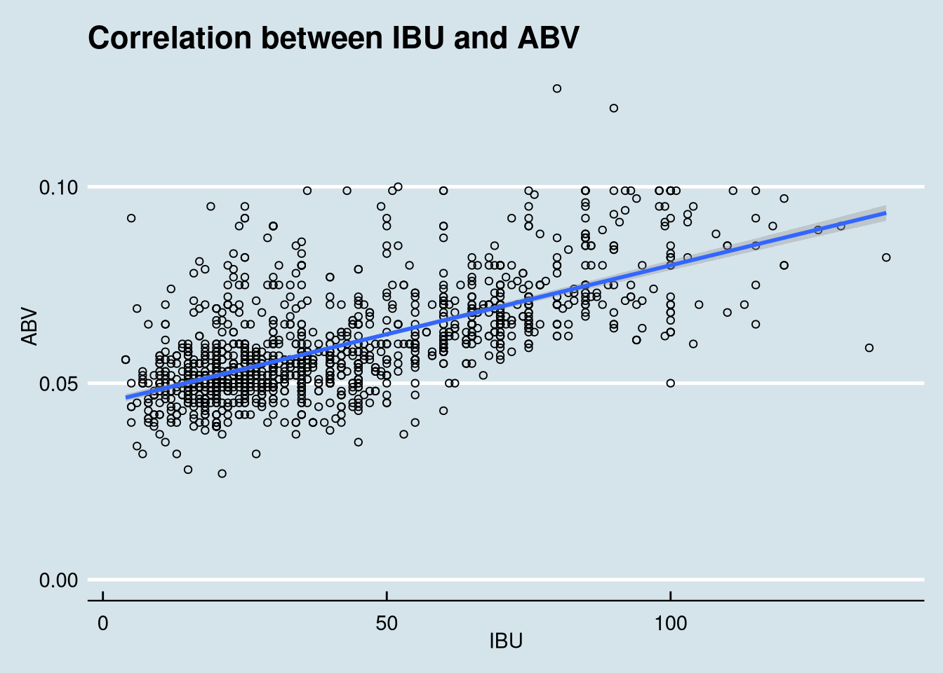

cor.test(Brewdata$IBU, Brewdata$ABV)

## 
##  Pearson's product-moment correlation
## 
## data:  Brewdata$IBU and Brewdata$ABV
## t = 33.848, df = 1401, p-value < 2.2e-16
## alternative hypothesis: true correlation is not equal to 0
## 95 percent confidence interval:
##  0.6408842 0.6985369
## sample estimates:
##       cor 
## 0.6707224

It appears that there is some correlation between bitterness and ABV. The data shows a trend that generally as bitterness increases, so does alcohol content. However, alcohol content may increase with or without an increase in bitterness.

Several of the highly bitter beers have considerably more alcohol in them than thier less bitter counterparts.
Pearson’s R = .6706
Pearson’s 𝑅^2 = 45%

There is sufficient evidence (p-value <.0001) that the alcohol by volume (ABV) and International Bittering Units (IBU) are linearly correlated. We estimate that 45% of the variation in ABV is explained by IBU.

8. Investigate the difference with respect to IBU and ABV between IPAs (India Pale Ales) and other types of Ale (any beer with “Ale” in its name other than IPA). We will use KNN to classify each ‘ale’ as either an IPA or Other and provide statistical evidence to back up this claim.

Brewdata.impute.draft <- Brewdata.impute.draft %>% dplyr::rename(ABV.New = ABV)
Brewdata.impute.draft <- Brewdata.impute.draft %>% dplyr::rename(IBU.New = IBU)
Brewdata.New <- full_join(Brewdata, Brewdata.impute.draft, by = "Beer_ID")

Ales.beer <- cbind(Brewdata.New, type='Ales', stringsAsFactors=F) %>% filter(grepl('\\bale\\b', Style, ignore.case=T))
IPA.beer <- cbind(Brewdata.New, type='IPA', stringsAsFactors=F) %>% filter(grepl('\\bIPA\\b', Style, ignore.case=T))
IPA.Ales <- union(Ales.beer, IPA.beer)
IPA.Ales$type <- as.factor(IPA.Ales$type)

set.seed(100)
splitPerc = .7
iterations = 100
numks =50
masterAcc = matrix(nrow = iterations, ncol = numks)

for(j in 1:iterations) {
  
  accs = data.frame(accuracy = numeric(numks), k = numeric(numks))
  trainIndices = sample(1:dim(IPA.Ales)[1],round(splitPerc * dim(IPA.Ales)[1]))
  train = IPA.Ales[trainIndices,]
  test = IPA.Ales[-trainIndices,]
  
  for(i in 1:numks) {
    
    classifications = knn(train[,c('IBU.New','ABV.New')],test[,c('IBU.New','ABV.New')],as.factor(train$type), prob = TRUE, k = i)
    
    table(as.factor(test$type),classifications)
    CM = confusionMatrix(table(as.factor(test$type),classifications))
    masterAcc[j,i] = CM$overall[1]
  }
}

MeanAcc = colMeans(masterAcc)
plot(seq(1,numks,1),MeanAcc, type = "l")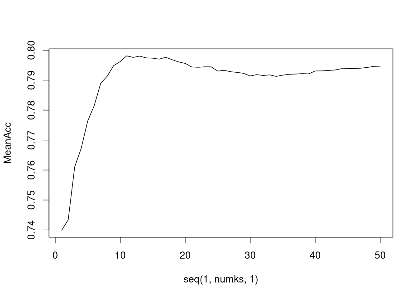

k <- which.max(MeanAcc)

classifications = knn(train[,c('IBU.New','ABV.New')],test[,c('IBU.New','ABV.New')],train$type, prob = TRUE, k)

table(test$type,classifications)

##       classifications
##        Ales IPA
##   Ales  249  39
##   IPA    61 115

confusionMatrix(table(test$type,classifications))

## Confusion Matrix and Statistics
## 
##       classifications
##        Ales IPA
##   Ales  249  39
##   IPA    61 115
##                                           
##                Accuracy : 0.7845          
##                  95% CI : (0.7442, 0.8211)
##     No Information Rate : 0.6681          
##     P-Value [Acc > NIR] : 2.294e-08       
##                                           
##                   Kappa : 0.5309          
##                                           
##  Mcnemar's Test P-Value : 0.03573         
##                                           
##             Sensitivity : 0.8032          
##             Specificity : 0.7468          
##          Pos Pred Value : 0.8646          
##          Neg Pred Value : 0.6534          
##              Prevalence : 0.6681          
##          Detection Rate : 0.5366          
##    Detection Prevalence : 0.6207          
##       Balanced Accuracy : 0.7750          
##                                           
##        'Positive' Class : Ales            
##

9. Additional Research.

# Reset Datafiles:
breweries <- read.csv("./data/Breweries.csv", header = TRUE, strip.white=TRUE)
beers <- read.csv("./data/Beers.csv", header = TRUE)
beers <-  beers %>% dplyr::rename( Brew_ID = Brewery_id)
breweries <- breweries %>% dplyr::rename(Name_Brew = Name)  
beers <- beers %>% dplyr::rename(Name_Beer = Name)
brew.beer <- full_join(breweries, beers, by = "Brew_ID")
brew.beerABVper <- mutate(brew.beer, ABVper = ABV * 100)

# Build regional info:
brew.beerABVper$Region[brew.beerABVper$State == "ME"] <- "Northeast"
brew.beerABVper$Region[brew.beerABVper$State == "NH"] <- "Northeast"
brew.beerABVper$Region[brew.beerABVper$State == "VT"] <- "Northeast"
brew.beerABVper$Region[brew.beerABVper$State == "MA"] <- "Northeast"
brew.beerABVper$Region[brew.beerABVper$State == "RI"] <- "Northeast"
brew.beerABVper$Region[brew.beerABVper$State == "CT"] <- "Northeast"
brew.beerABVper$Region[brew.beerABVper$State == "NY"] <- "Northeast"
brew.beerABVper$Region[brew.beerABVper$State == "NJ"] <- "Northeast"
brew.beerABVper$Region[brew.beerABVper$State == "PA"] <- "Northeast"
brew.beerABVper$Region[brew.beerABVper$State == "ND"] <- "Midwest"
brew.beerABVper$Region[brew.beerABVper$State == "SD"] <- "Midwest"
brew.beerABVper$Region[brew.beerABVper$State == "NE"] <- "Midwest"
brew.beerABVper$Region[brew.beerABVper$State == "KS"] <- "Midwest"
brew.beerABVper$Region[brew.beerABVper$State == "MN"] <- "Midwest"
brew.beerABVper$Region[brew.beerABVper$State == "IA"] <- "Midwest"
brew.beerABVper$Region[brew.beerABVper$State == "MO"] <- "Midwest"
brew.beerABVper$Region[brew.beerABVper$State == "WI"] <- "Midwest"
brew.beerABVper$Region[brew.beerABVper$State == "IL"] <- "Midwest"
brew.beerABVper$Region[brew.beerABVper$State == "IN"] <- "Midwest"
brew.beerABVper$Region[brew.beerABVper$State == "MI"] <- "Midwest"
brew.beerABVper$Region[brew.beerABVper$State == "OH"] <- "Midwest"
brew.beerABVper$Region[brew.beerABVper$State == "OK"] <- "South"
brew.beerABVper$Region[brew.beerABVper$State == "TX"] <- "South"
brew.beerABVper$Region[brew.beerABVper$State == "AR"] <- "South"
brew.beerABVper$Region[brew.beerABVper$State == "LA"] <- "South"
brew.beerABVper$Region[brew.beerABVper$State == "MS"] <- "South"
brew.beerABVper$Region[brew.beerABVper$State == "KY"] <- "South"
brew.beerABVper$Region[brew.beerABVper$State == "TN"] <- "South"
brew.beerABVper$Region[brew.beerABVper$State == "AL"] <- "South"
brew.beerABVper$Region[brew.beerABVper$State == "FL"] <- "South"
brew.beerABVper$Region[brew.beerABVper$State == "GA"] <- "South"
brew.beerABVper$Region[brew.beerABVper$State == "SC"] <- "South"
brew.beerABVper$Region[brew.beerABVper$State == "NC"] <- "South"
brew.beerABVper$Region[brew.beerABVper$State == "VA"] <- "South"
brew.beerABVper$Region[brew.beerABVper$State == "WV"] <- "South"
brew.beerABVper$Region[brew.beerABVper$State == "MD"] <- "South"
brew.beerABVper$Region[brew.beerABVper$State == "DE"] <- "South"
brew.beerABVper$Region[brew.beerABVper$State == "WA"] <- "West"
brew.beerABVper$Region[brew.beerABVper$State == "OR"] <- "West"
brew.beerABVper$Region[brew.beerABVper$State == "CA"] <- "West"
brew.beerABVper$Region[brew.beerABVper$State == "AK"] <- "West"
brew.beerABVper$Region[brew.beerABVper$State == "HI"] <- "West"
brew.beerABVper$Region[brew.beerABVper$State == "AZ"] <- "West"
brew.beerABVper$Region[brew.beerABVper$State == "NV"] <- "West"
brew.beerABVper$Region[brew.beerABVper$State == "ID"] <- "West"
brew.beerABVper$Region[brew.beerABVper$State == "MT"] <- "West"
brew.beerABVper$Region[brew.beerABVper$State == "WY"] <- "West"
brew.beerABVper$Region[brew.beerABVper$State == "CO"] <- "West"
brew.beerABVper$Region[brew.beerABVper$State == "NM"] <- "West"
brew.beerABVper$Region[brew.beerABVper$State == "UT"] <- "West"

Compare Region, City and Brewery Stats

# Calculate mean ABV by Region
bbABVper.clean <- brew.beerABVper %>% filter(!is.na(brew.beerABVper$ABVper))
bbABVper.cleanmea <- aggregate(bbABVper.clean$ABVper, by=list(bbABVper.clean$Region), FUN = mean)
colnames(bbABVper.cleanmea) <- c("Region", "MeanABV")
bbABVper.cleanmea$MeanABV <- round(bbABVper.cleanmea$MeanABV, 2)

# Calculate mean IBU by Region
bbIBU.clean <- brew.beerABVper %>% filter(!is.na(brew.beerABVper$IBU))
bbIBU.cleanmed <- aggregate(bbIBU.clean$IBU, by=list(bbIBU.clean$Region), FUN = median)
colnames(bbIBU.cleanmed) <- c("Region", "MedianIBU")
bbIBU.cleanmea <- aggregate(bbIBU.clean$IBU, by=list(bbIBU.clean$Region), FUN = mean)
colnames(bbIBU.cleanmea) <- c("Region", "MeanIBU")

# Calculate Top 10 Cities with the most Breweries
TopCities <- Brewdata %>% mutate(City = paste0(City, ', ', state)) %>% group_by(City) %>% 
  summarise(Breweries = n()) %>% arrange(desc(Breweries))

# Calculate Top 10 Breweries with the most original beers
TopBreweries <- Brewdata %>% mutate(Brewery = paste0(Brewery,'<br>', City, ', ', state)) %>% 
  group_by(Brewery) %>% summarise(Beers = n()) %>% arrange(desc(Beers))

Top10Cities <- top_n(TopCities,10)

## Selecting by Breweries

Top10Breweries <- top_n(TopBreweries,10)

## Selecting by Beers

Build the plots

charts <- list()
charts[['zero']] <- ''

charts[['meanABVbyRegion']] <-
hchart(bbABVper.cleanmea, "column", hcaes(x = Region, y = MeanABV)) %>% 
  hc_title(text = "Average ABV by Region") %>%
  hc_add_theme(hc_theme_economist())

charts[['MedianIBUbyRegion']] <-
hchart(bbIBU.cleanmed, "column", hcaes(x = Region, y = MedianIBU)) %>% 
  hc_title(text = "Median IBU by Region") %>%
  hc_add_theme(hc_theme_economist())

charts[['top10byCity']] <-
hchart(Top10Cities, "column", hcaes(x = City, y = Breweries)) %>% 
  hc_title(text = "Top 10 Cities with Most Breweries") %>%
  hc_add_theme(hc_theme_economist())

charts[['top10byBrewery']] <-
hchart(Top10Breweries, "column", hcaes(x = Brewery, y = Beers)) %>% 
  hc_title(text = "Top 10 Breweries with Most Original Beers") %>%
  hc_add_theme(hc_theme_economist())


  #  TopBreweries <- Brewdata %>% mutate(Brewery = paste0(Brewery,'<br>', City, ', ', state)) %>% 
  #  group_by(Brewery) %>% summarise(Beers = n()) %>% arrange(desc(Beers))
   # ggplot(data=Brewdata, mapping=aes(x=Brewery, y=Beers)) + geom_col() + theme_economist() + 
   # labs(title = "Top 10 Breweries with Most Original Beers")

Visualization of our additional research!

htmltools::tagList(charts)

 #   TopBreweries <- Brewdata %>% mutate(Brewery = paste0(Brewery,'\n', City, ', ', state)) %>% 
  #  group_by(Brewery) %>% summarise(Beers = n()) %>% arrange(desc(Beers)) %>% top_n(10)
  #  ggplot(data=TopBreweries, mapping=aes(x=Brewery, y=Beers)) + geom_col(color="white",fill="steelblue") +
  #    theme_economist()  +labs(title = "Top 10 Breweries with Most Original Beers") +
   #   theme(axis.text.x = element_text(angle = 60, vjust=1, hjust=1))