Employee Attrition Data Analysis
Dustin Bracy
12/05/2019
Abstract:
DDSAnalytics is an analytics company that specializes in talent management solutions for Fortune 100 companies. Talent management is the iterative process of developing and retaining employees. To gain a competitive edge over its competition, DDSAnalytics is planning to leverage data science for talent management. The executive leadership has identified predicting employee turnover as its first application of data science for talent management. Before the business green lights the project, they have tasked my data science team to conduct an analysis of existing employee data.
Objectives:
- Identify the top three factors that contribute to employee attrition (backed up by evidence provided by data analysis).
- Identify job and/or role specific trends.
- Identify useful factors related to talent management (e.g. workforce planning, employee training, identifying high potential employees, reducing turnover).
- Present findings via YouTube in 7 minutes or less.
Target Audience:
- Client CEO and CFO
- CEO is statistician, CFO has had only one class in statistics
Data Analysis & Findings:
- training times last year indicates the number of training sessions attended
- hourly/daily/monthly rates are unclear, possibly production rates
- Ordinal scales where used indicate 1 as low/worst, and 5 as high/best
- Performance ratings seem to indicate a fear of giving a low score (possible company culture issue)
- Only 3s and 4s were given, no 1 or 2s
- SalesRepresentatives have the highest attrition rate, and Directors have the lowest
- Job Level, Total Working Years, and Years at Company have the most impact on Monthly Income
- Overtime, no stock options, and employees in low level jobs (level 1) are the biggest drivers of attrition
- Employees making less that $5,000 per month have the highest attrition rates
- Employees under 30 are more likely to leave their jobs
- Employees with less than 5 years at a company or 5 total working years are more likely to leave
Import & Validate data:
A simple sum of missing values returns 0, which means this dataset is clean and we can start our EDA!
Exploratory Data Analysis
In Exploratory Data Analysis (EDA), we’re looking for correlation among 36 original features. We are primarily looking for features that we can use to predict attrition in the workplace.
data <- read.csv("./data/CaseStudy2-data.csv", header=T)
#data <- read.csv("./data/CaseStudy2CompSet No Attrition.csv", header=T)
oData <- data # Save original dataset

# Check for missing values:
MissingValues <- sapply(data, function(x) sum(is.na(x)))
sum(MissingValues)
## [1] 0# One-hot encode categorical variables:
data$Attrition <- ifelse(data$Attrition == "Yes",1,0)
data$OverTime <- ifelse(data$OverTime == "Yes",1,0)
data$Gender <- ifelse(data$Gender == "Male",1,0)
data$BusinessTravel <- as.numeric(factor(data$BusinessTravel,
levels=c("Non-Travel", "Travel_Rarely", "Travel_Frequently"))) -1
data$HumanResources <- ifelse(data$Department == "Human Resources",1,0)
data$ResearchDevelopment <- ifelse(data$Department == "Research & Development",1,0)
data$Sales <- ifelse(data$Department == "Sales",1,0)
data$Single <- ifelse(data$MaritalStatus == "Single",1,0)
data$Married <- ifelse(data$MaritalStatus == "Married",1,0)
data$Divorced <- ifelse(data$MaritalStatus == "Divorced",1,0)
data$EdHumanResources <- ifelse(data$EducationField == "Human Resources",1,0)
data$EdLifeSciences <- ifelse(data$EducationField == "Life Sciences",1,0)
data$EdMedical <- ifelse(data$EducationField == "Medical",1,0)
data$EdMarketing <- ifelse(data$EducationField == "Marketing",1,0)
data$EdTechnicalDegree <- ifelse(data$EducationField == "Technical Degree",1,0)
data$EdOther <- ifelse(data$EducationField == "Other",1,0)
data$JobSalesExecutive <- ifelse(data$JobRole == "Sales Executive",1,0)
data$JobResearchDirector <- ifelse(data$JobRole == "Research Director",1,0)
data$JobManufacturingDirector <- ifelse(data$JobRole == "Manufacturing Director",1,0)
data$JobResearchScientist <- ifelse(data$JobRole == "Research Scientist",1,0)
data$JobSalesExecutive <- ifelse(data$JobRole == "Sales Executive",1,0)
data$JobSalesRepresentative <- ifelse(data$JobRole == "Sales Representative",1,0)
data$JobManager <- ifelse(data$JobRole == "Manager",1,0)
data$JobHealthcareRepresentative <- ifelse(data$JobRole == "Healthcare Representative",1,0)
data$JobHumanResources <- ifelse(data$JobRole == "Human Resources",1,0)
data$JobLaboratoryTechnician <- ifelse(data$JobRole == "Laboratory Technician",1,0)Continuous Data:
# Visualize continuous data:
pIncome <- data %>% ggplot(aes(MonthlyIncome, Attrition)) + geom_smooth()
pDistance <- data %>% ggplot(aes(DistanceFromHome, Attrition)) + geom_smooth()
pSalaryHike <- data %>% ggplot(aes(PercentSalaryHike, Attrition)) + geom_smooth()
pCompanies <- data %>% ggplot(aes(NumCompaniesWorked, Attrition)) + geom_smooth()
pDaily <- data %>% ggplot(aes(DailyRate, Attrition)) + geom_smooth()
pHourly <- data %>% ggplot(aes(HourlyRate, Attrition)) + geom_smooth()
pMonthly <- data %>% ggplot(aes(MonthlyRate, Attrition)) + geom_smooth()
pAge <- data %>% ggplot(aes(Age, Attrition)) + geom_smooth()
pYearsCompany <- data %>% ggplot(aes(YearsAtCompany, Attrition)) + geom_smooth()
pYearsRole <- data %>% ggplot(aes(YearsInCurrentRole, Attrition)) + geom_smooth()
pPromotion <- data %>% ggplot(aes(YearsSinceLastPromotion, Attrition)) + geom_smooth()
pYearsManager <- data %>% ggplot(aes(YearsWithCurrManager, Attrition)) + geom_smooth()
pYearsWorking <- data %>% ggplot(aes(TotalWorkingYears, Attrition)) + geom_smooth()
grid.arrange(pIncome,pDistance,pSalaryHike,pCompanies,pDaily,pHourly,pMonthly,pAge,pYearsCompany,pYearsRole,pPromotion,pYearsManager,pYearsWorking, ncol=4, nrow=4)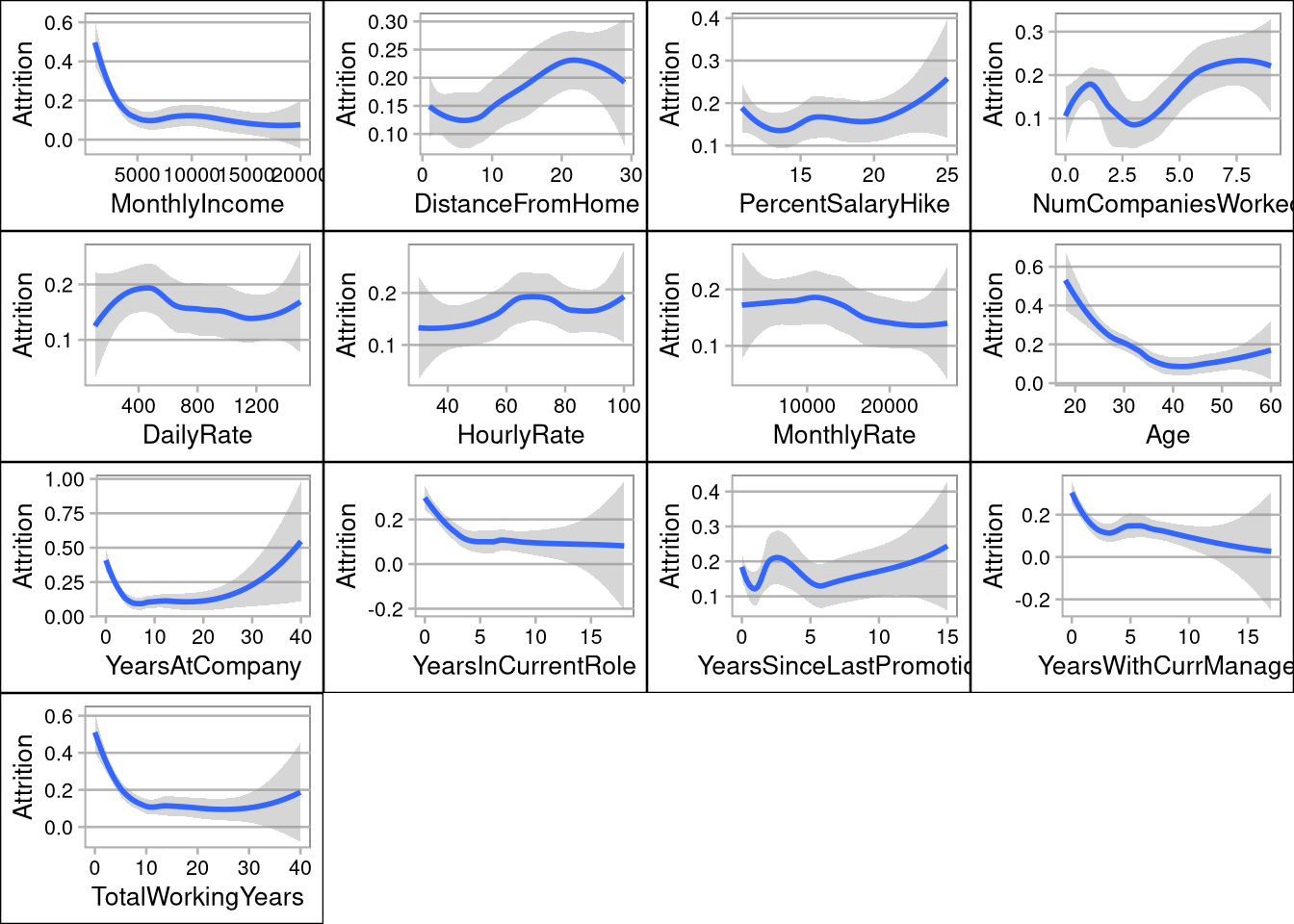
Ordinal Data:
# Visualize ordinal data:
pJobSat <- data %>% ggplot(aes(JobSatisfaction, Attrition)) + geom_smooth()
pJobLevel <- data %>% ggplot(aes(JobLevel, Attrition)) + geom_smooth()
pJobInvolvement <- data %>% ggplot(aes(JobInvolvement, Attrition)) + geom_smooth()
pTraining <- data %>% ggplot(aes(TrainingTimesLastYear, Attrition)) + geom_smooth()
pStock <- data %>% ggplot(aes(StockOptionLevel, Attrition)) + geom_smooth()
pTravel <- data %>% ggplot(aes(BusinessTravel, Attrition)) + geom_smooth()
pEducation <- data %>% ggplot(aes(Education, Attrition)) + geom_smooth()
pRelationship <- data %>% ggplot(aes(RelationshipSatisfaction, Attrition)) + geom_smooth()
pWorkLife <- data %>% ggplot(aes(WorkLifeBalance, Attrition)) + geom_smooth()
grid.arrange(pJobSat,pJobLevel,pJobInvolvement,pTraining,pStock,pTravel,pEducation,pRelationship,pWorkLife, ncol=3, nrow=3)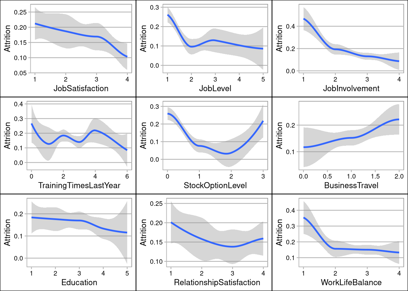
Categorical Data:
# Visualize categorical data:
pAttrition <- oData %>% group_by(Attrition) %>% summarise(count = n()) %>%
    mutate(Percent = (count / sum(count))*100) %>%
    ggplot() + geom_bar(aes(y=Percent, x=Attrition, fill=Attrition), stat = "identity")
pDept <- oData %>% ggplot(aes(Department, fill=Attrition)) + geom_bar()  + coord_flip()
pMarital <- oData %>% ggplot(aes(MaritalStatus, fill=Attrition)) + geom_bar()
pGender <- oData %>% ggplot(aes(Gender, fill=Attrition)) + geom_bar()
grid.arrange(pAttrition, pDept, pMarital,pGender, ncol=2, nrow=2)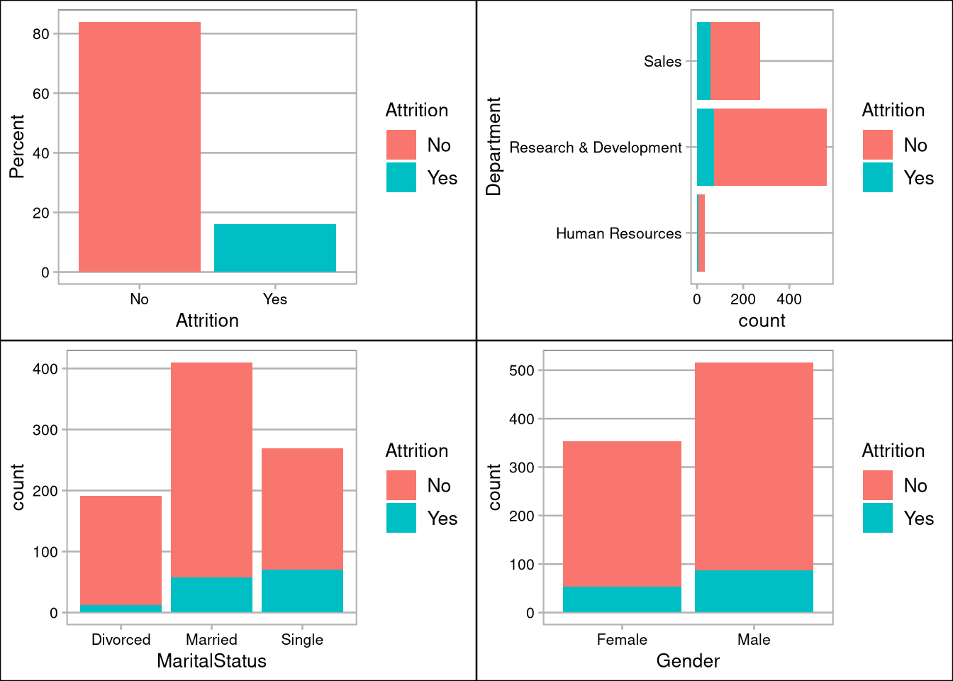
oData %>% ggplot(aes(JobRole, fill=Attrition)) + geom_bar() + coord_flip() + coord_flip() + labs(title="Attrition by Job Role", y="Employees")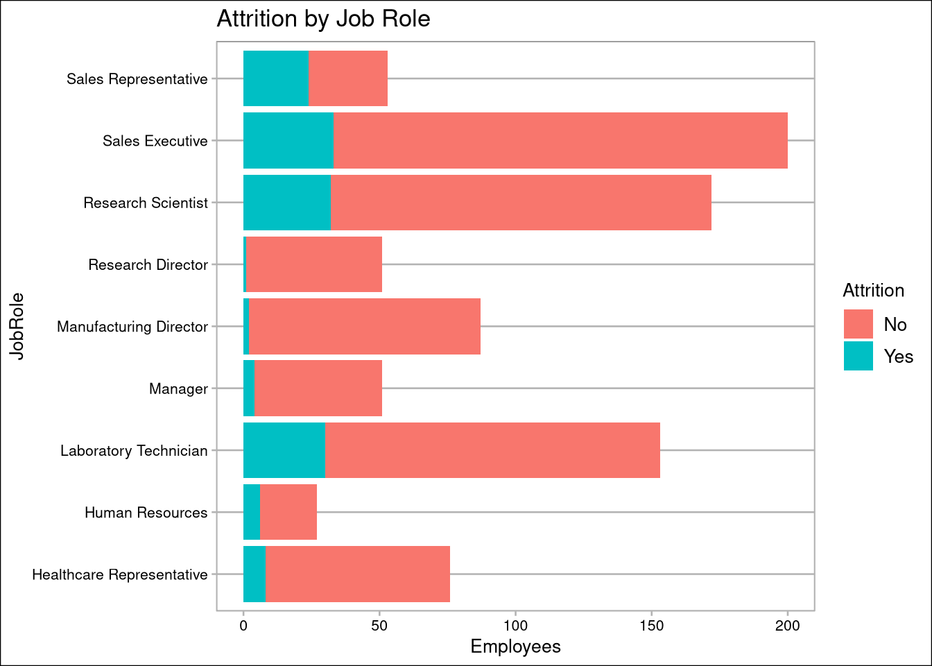
oData %>% ggplot(aes(EducationField)) + geom_bar(aes(fill=Attrition)) + coord_flip() + labs(title="Attrition by Educational Field", y="Employees")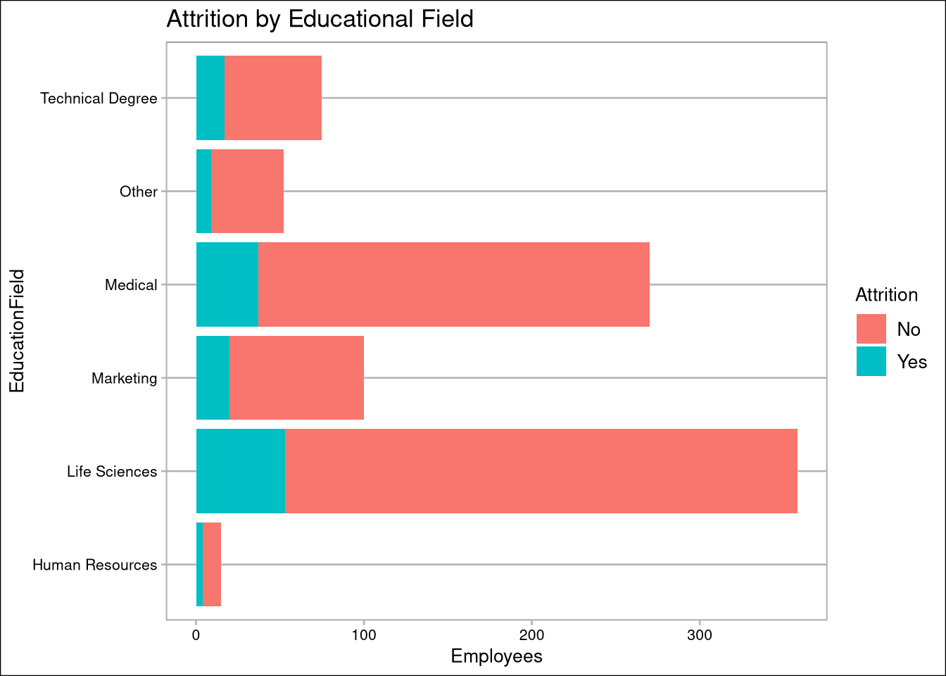
Feature Engineering
Feature engineering is designed to improve correlation by combining like type features, or slicing the data into distinct populations. I am going to use it to binary encode the categorical data to allow me to use Logistical Regression and improve performance in the KNN algorithm while predicting employee attrition and salary.
# binary encode ordinal variables
data$LessThan5k <- ifelse(data$MonthlyIncome < 5000, 1, 0)
data$NewWorker <- ifelse(data$NumCompaniesWorked <=1, 1, 0)
data$LowLevel <- ifelse(data$JobLevel == 1, 1, 0)
data$NewHire <- ifelse(data$YearsAtCompany <4, 1, 0)
data$WorkedOver30 <- ifelse(data$TotalWorkingYears >=30, 1, 0)
data$Uninvolved <- ifelse(data$JobInvolvement <2, 1, 0)
data$NewToRole <- ifelse(data$YearsInCurrentRole <=1, 1, 0)
data$Unbalanced <- ifelse(data$WorkLifeBalance <2, 1, 0)
data$SalaryHike <- ifelse(data$PercentSalaryHike  >20, 1, 0)
data$HighlySatisfied <- ifelse(data$JobSatisfaction == 4, 1, 0)
data$LongCommute <- ifelse(data$DistanceFromHome >= 15, 1, 0)
data$AgeUnder40 <- ifelse(data$Age <40, 1, 0)
data$DueForPromotion <- ifelse(!data$YearsSinceLastPromotion %in% c(1,5,6,7), 1, 0)
data$TopPerformer <- ifelse(data$PerformanceRating == 4, 1, 0)
data$NoStock <- ifelse(data$StockOptionLevel < 1, 1 , 0)
data$NoTraining <- ifelse(data$TrainingTimesLastYear < 1, 1, 0)
data$HourlyOver40 <- ifelse(data$HourlyRate > 40, 1, 0)
data$MonthlyOver15k <- ifelse(data$MonthlyRate > 15000, 1, 0)
data$LogIncome <- log(data$MonthlyIncome)
data$SqIncome <- data$MonthlyIncome^2
data$SqRtIncome <- sqrt(data$MonthlyIncome)


# drop factors for regression analysis
rdata <- subset(data, select = -c(Over18, Department, JobRole, MaritalStatus, EducationField, EmployeeCount, StandardHours))

# scale numerics 0-1 to improve KNN performance
kdata <- data.frame(apply(rdata, MARGIN = 2, FUN = function(X) (X - min(X))/diff(range(X))))

# set the test/train split
splitPerc <- .7
Correlation Analysis
Here we are looking to see improvement gained from feature engineering and to ensure we select features which have high correlation with our response variables (i.e. Income/Attrition) for use in our machine learning algorthims.

Correlation Plot of all Rdata features
data.cor <- cor(rdata)
cdata <- data.cor[,c('Attrition','MonthlyIncome')]
cdata <- data.frame(rbind(names(cdata),cdata))
cdata <- tibble::rownames_to_column(cdata, "Feature")
IncomeCorrelation <- cdata %>% select(Feature, MonthlyIncome) %>% filter(!Feature %in% c('MonthlyIncome',"LogIncome","SqIncome","SqRtIncome")) %>% arrange(abs(MonthlyIncome))

AttritionCorrelation <- cdata %>% select(Feature, Attrition) %>% arrange(abs(Attrition)) %>% filter(Feature != 'Attrition' )
AttritionCorrelation$Feature <- as.factor(AttritionCorrelation$Feature)
IncomeCorrelation %>% top_n(10) %>% mutate(Feature = factor(Feature, Feature)) %>%
ggplot(aes(Feature,MonthlyIncome, fill=Feature)) +
geom_col() + labs(title="Top 10 Monthly Income Drivers") + coord_flip() +
scale_fill_discrete(guide = guide_legend(reverse=TRUE))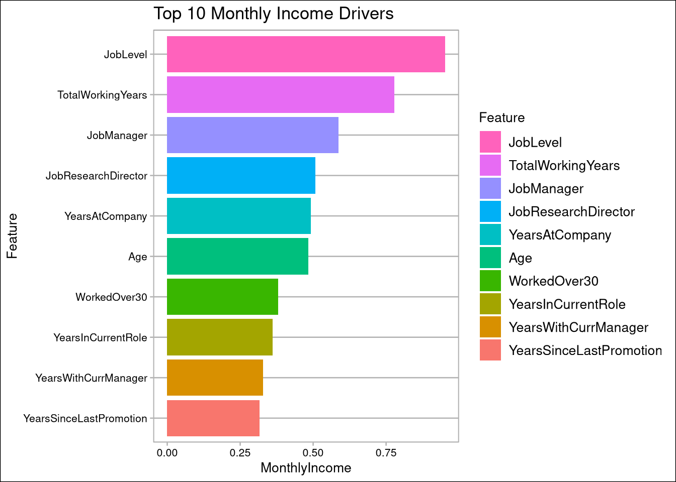
AttritionCorrelation  %>% top_n(10) %>% mutate(Feature = factor(Feature, Feature)) %>%
  ggplot(aes(Feature,Attrition, fill=Feature)) + geom_col() +
  labs(title="Top 10 Attrition Drivers") + coord_flip() +
  scale_fill_discrete(guide = guide_legend(reverse=TRUE))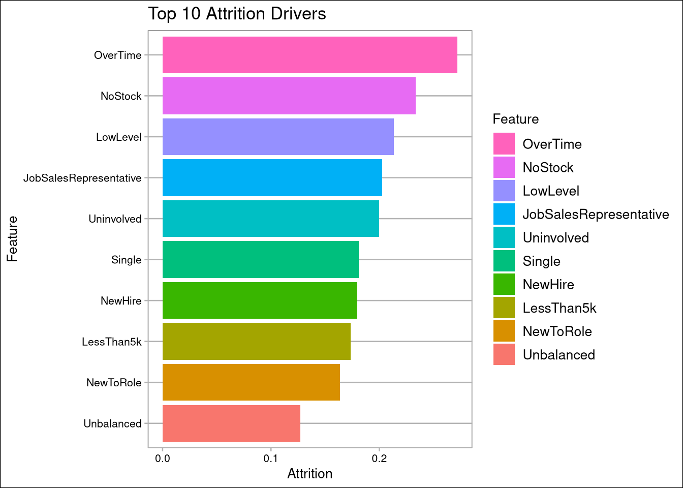
# View correlation for KNN prediction:
data %>% select(
  'Attrition',
  "JobSatisfaction",
  "OverTime",
  "WorkLifeBalance",
  "JobInvolvement",
  "NewHire",
  "DueForPromotion",
  "NoStock",
  "DistanceFromHome",
  "MonthlyIncome"
  ) %>% ggpairs(title = "Correlation for Attrition using KNN Features")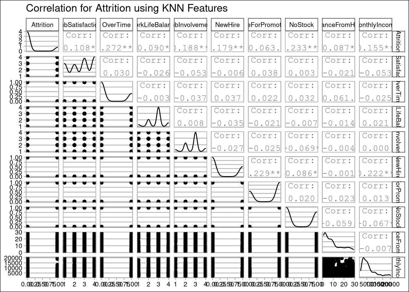
# View correlation plots for salary regression:
data %>% select(
   'MonthlyIncome',
   'JobLevel',
   'TotalWorkingYears',
   'JobRole'
   ) %>% ggpairs(title = "Correlation for Monthly Income using Linear Regression Features")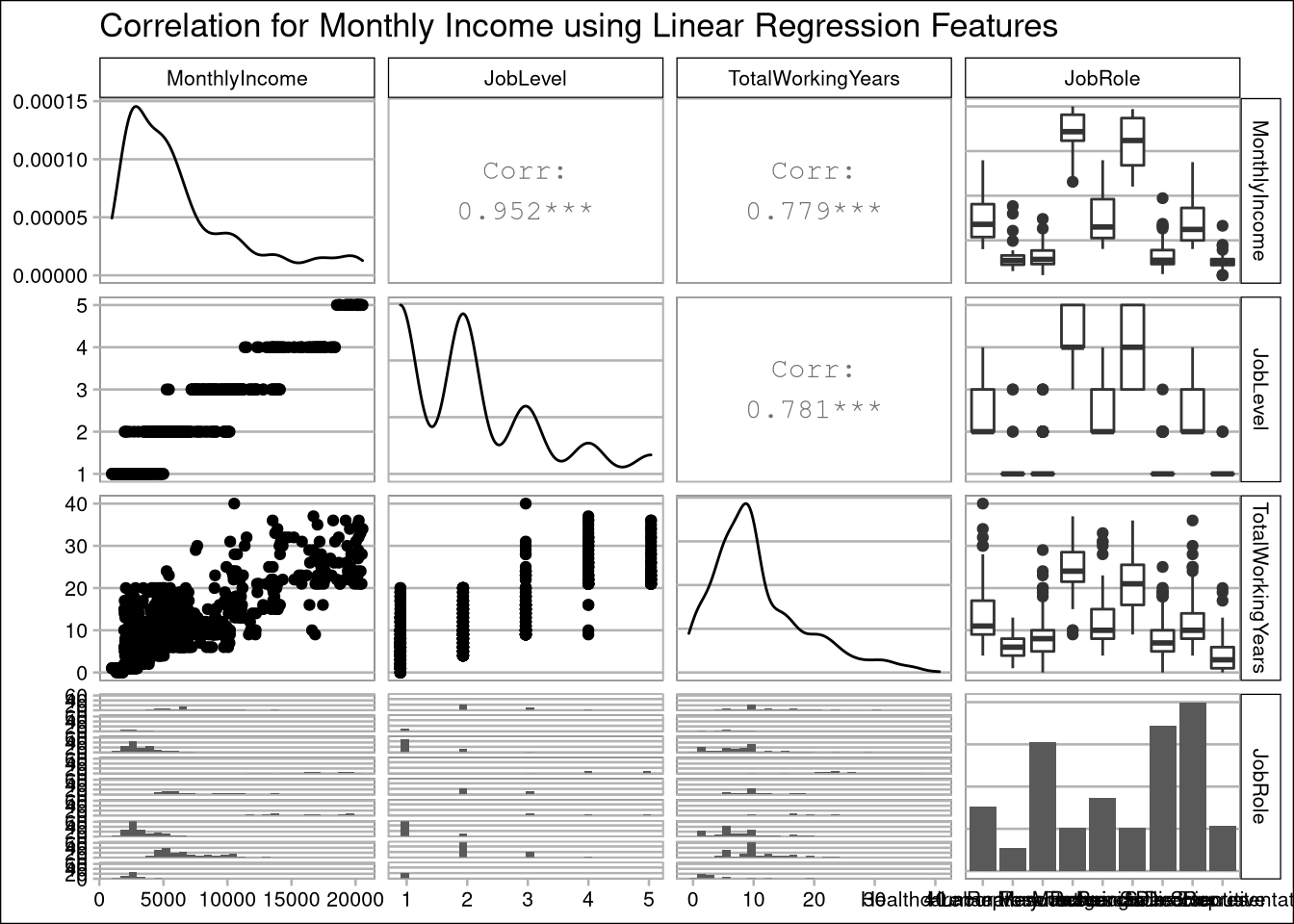
Using K Nearest Neighbors (KNN) to predict employee attrition
First we need to determine the best value of K to use for KNN. We use 50 iterations of tests across all 35 values of K (120% of the square root of the size of the dataset) to find the max useful value of K and the average of its performance statistics.
iterations = 50
set.seed(7)
numks = round(sqrt(dim(kdata)[1])*1.2)
masterAcc = matrix(nrow = iterations, ncol = numks)
masterSpec = matrix(nrow = iterations, ncol = numks)
masterSen = matrix(nrow = iterations, ncol = numks)
knnArray <- c("JobSatisfaction",
              "OverTime",
              "WorkLifeBalance",
              "JobInvolvement",
              "NewHire",
              "DueForPromotion",
              "NoStock",
              "DistanceFromHome",
              "MonthlyIncome"
              )

for(j in 1:iterations) {
  # resample data
  trainIndices = sample(1:dim(kdata)[1],round(splitPerc * dim(kdata)[1]))
  train = kdata[trainIndices,]
  test = kdata[-trainIndices,]
  for(i in 1:numks) {
    # predict using i-th value of k
    classifications = knn(train[,knnArray],test[,knnArray],as.factor(train$Attrition), prob = TRUE, k = i)
    CM = confusionMatrix(table(as.factor(test$Attrition),classifications, dnn = c("Prediction", "Reference")), positive = '1')
    masterAcc[j,i] = CM$overall[1]
    masterSen[j,i] = CM$byClass[1]
    masterSpec[j,i] = ifelse(is.na(CM$byClass[2]),0,CM$byClass[2])

  }
}

MeanAcc <- colMeans(masterAcc)
MeanSen <- colMeans(masterSen)
MeanSpec <- colMeans(masterSpec)
plot(seq(1,numks), MeanAcc, main="K value determination", xlab="Value of K")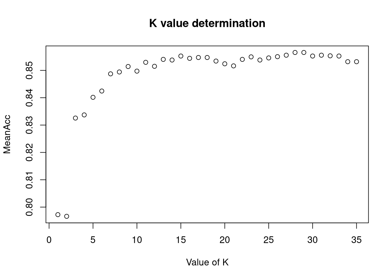
k <- which.max(MeanAcc)
specs <- c(MeanAcc[k],MeanSen[k],MeanSpec[k])
names(specs) <- c("Avg Accuracy", "Avg Sensitivity", "Avg Specificity")
specs %>% kable("html") %>% kable_styling | x | |
|---|---|
| Avg Accuracy | 0.8565517 |
| Avg Sensitivity | 0.6782740 |
| Avg Specificity | 0.8661193 |
classifications = knn(train[,knnArray],test[,knnArray],as.factor(train$Attrition), prob = TRUE, k = k)
confusionMatrix(table(test$Attrition,classifications, dnn = c("Prediction", "Reference")), positive = '1')
## Confusion Matrix and Statistics
##
## Reference
## Prediction 0 1
## 0 215 6
## 1 28 12
##
## Accuracy : 0.8697
## 95% CI : (0.8227, 0.9081)
## No Information Rate : 0.931
## P-Value [Acc > NIR] : 0.9998644
##
## Kappa : 0.3522
##
## Mcnemar's Test P-Value : 0.0003164
##
## Sensitivity : 0.66667
## Specificity : 0.88477
## Pos Pred Value : 0.30000
## Neg Pred Value : 0.97285
## Prevalence : 0.06897
## Detection Rate : 0.04598
## Detection Prevalence : 0.15326
## Balanced Accuracy : 0.77572
##
## 'Positive' Class : 1
## Using Naive Bayes to predict employee attrition
Naive Bayes uses 100 iterations to find an average performance statistics.
iterations = 100
set.seed(7)
masterAcc = matrix(nrow = iterations)
masterSpec = matrix(nrow = iterations)
masterSen = matrix(nrow = iterations)

nbArray <- c("HighlySatisfied",
             "OverTime",
             "LowLevel",
             "Unbalanced",
             "WorkedOver30",
             "JobInvolvement",
             "SalaryHike",
             "NewHire",
             "NewToRole",
             "AgeUnder40",
             "DueForPromotion",
             "TopPerformer",
             "NoStock",
             "MaritalStatus",
             "LogIncome",
             "MonthlyOver15k",
             "HourlyOver40")

nbArray <- knnArray

for(j in 1:iterations)
{

  trainIndices = sample(1:dim(data)[1],round(splitPerc * dim(data)[1]))
  train = data[trainIndices,]
  test = data[-trainIndices,]
  model = naiveBayes(train[,nbArray],as.factor(train$Attrition),laplace = .0001)
  CM = confusionMatrix(table(predict(model,test[,nbArray]),as.factor(test$Attrition), dnn = c("Prediction", "Reference")), positive = '1')
  masterAcc[j] = CM$overall[1]
  masterSen[j] = CM$byClass[1]
  masterSpec[j] = CM$byClass[2]

}
specs <- c(colMeans(masterAcc),colMeans(masterSen),colMeans(masterSpec))
names(specs) <- c("Avg Accuracy", "Avg Sensitivity", "Avg Specificity")
specs %>% kable("html") %>% kable_styling | x | |
|---|---|
| Avg Accuracy | 0.8617241 |
| Avg Sensitivity | 0.4044971 |
| Avg Specificity | 0.9505032 |
confusionMatrix(table(predict(model,test[,nbArray]),as.factor(test$Attrition), dnn = c("Prediction", "Reference")), positive = '1')## Confusion Matrix and Statistics
##
## Reference
## Prediction 0 1
## 0 195 28
## 1 18 20
##
## Accuracy : 0.8238
## 95% CI : (0.772, 0.868)
## No Information Rate : 0.8161
## P-Value [Acc > NIR] : 0.4115
##
## Kappa : 0.3613
##
## Mcnemar's Test P-Value : 0.1845
##
## Sensitivity : 0.41667
## Specificity : 0.91549
## Pos Pred Value : 0.52632
## Neg Pred Value : 0.87444
## Prevalence : 0.18391
## Detection Rate : 0.07663
## Detection Prevalence : 0.14559
## Balanced Accuracy : 0.66608
##
## 'Positive' Class : 1
## Using Fast Naive Bayes to predict employee attrition
The Fast Naive Bayes method below uses 100 iterations to find average performance statistics using only binary features.
iterations = 100
set.seed(7)
masterAcc2 = matrix(nrow = iterations)
masterSpec2 = matrix(nrow = iterations)
masterSen2 = matrix(nrow = iterations)

nbArray2 <- c("OverTime",
              "LowLevel",
              "HighlySatisfied",
              "Unbalanced",
              "WorkedOver30",
              "SalaryHike",
              "NewHire",
              "NewToRole",
              "AgeUnder40",
              "DueForPromotion",
              "TopPerformer",
              "NoStock",
              "Gender",
              "Uninvolved",
              "Single",
              "Divorced",
              "Married",
              "LongCommute",
              "NoTraining",
              "HourlyOver40",
              "MonthlyOver15k",
              "JobManager",
              "JobSalesExecutive",
              "JobSalesRepresentative")

for(j in 1:iterations)
{

  trainIndices = sample(1:dim(rdata)[1],round(splitPerc * dim(rdata)[1]))
  train2 = rdata[trainIndices,]
  test2 = rdata[-trainIndices,]
  model2 = fnb.bernoulli(train2[,nbArray2], train2$Attrition, laplace = .0001)
  CM2 = confusionMatrix(table(predict(model2,test2[,nbArray2]),as.factor(test2$Attrition), dnn = c("Prediction", "Reference")), positive = '1')
  masterAcc2[j] = CM2$overall[1]
  masterSen2[j] = CM2$byClass[1]
  masterSpec2[j] = CM2$byClass[2]
}
specs <- c(colMeans(masterAcc2),colMeans(masterSen2),colMeans(masterSpec2))
names(specs) <- c("Avg Accuracy", "Avg Sensitivity", "Avg Specificity")
specs %>% kable("html") %>% kable_styling | x | |
|---|---|
| Avg Accuracy | 0.8558238 |
| Avg Sensitivity | 0.4981112 |
| Avg Specificity | 0.9254531 |
confusionMatrix(table(predict(model2,test2[,nbArray2]),as.factor(test2$Attrition), dnn = c("Prediction", "Reference")), positive = '1')## Confusion Matrix and Statistics
##
## Reference
## Prediction 0 1
## 0 190 24
## 1 23 24
##
## Accuracy : 0.8199
## 95% CI : (0.7678, 0.8646)
## No Information Rate : 0.8161
## P-Value [Acc > NIR] : 0.4749
##
## Kappa : 0.3952
##
## Mcnemar's Test P-Value : 1.0000
##
## Sensitivity : 0.50000
## Specificity : 0.89202
## Pos Pred Value : 0.51064
## Neg Pred Value : 0.88785
## Prevalence : 0.18391
## Detection Rate : 0.09195
## Detection Prevalence : 0.18008
## Balanced Accuracy : 0.69601
##
## 'Positive' Class : 1
## Using Logistic Regression to predict employee attrition
set.seed(7)
trainIndices = sample(1:dim(data)[1],round(splitPerc * dim(data)[1]))
train = data[trainIndices,]
test = data[-trainIndices,]
model3 <- glm(Attrition ~ JobSatisfaction +
                OverTime +
                WorkLifeBalance +
                JobInvolvement +
                NewHire +
                NoStock +
                BusinessTravel +
                DistanceFromHome +
                YearsSinceLastPromotion +
                EnvironmentSatisfaction
              , data=train, family="binomial")

#HourlyRate+NewToRole +NumCompaniesWorked+LogIncome+JobRole
summary(model3)
##
## Call:
## glm(formula = Attrition ~ JobSatisfaction + OverTime + WorkLifeBalance +
## JobInvolvement + NewHire + NoStock + BusinessTravel + DistanceFromHome +
## YearsSinceLastPromotion + EnvironmentSatisfaction, family = "binomial",
## data = train)
##
## Deviance Residuals:
## Min 1Q Median 3Q Max
## -1.9646 -0.5692 -0.3528 -0.2028 2.9072
##
## Coefficients:
## Estimate Std. Error z value Pr(>|z|)
## (Intercept) -0.22404 0.81878 -0.274 0.78437
## JobSatisfaction -0.36064 0.11198 -3.220 0.00128 **
## OverTime 1.45197 0.25085 5.788 7.12e-09 ***
## WorkLifeBalance -0.30413 0.17454 -1.742 0.08143 .
## JobInvolvement -0.70384 0.17417 -4.041 5.32e-05 ***
## NewHire 1.09192 0.27736 3.937 8.26e-05 ***
## NoStock 1.21630 0.25697 4.733 2.21e-06 ***
## BusinessTravel 0.54487 0.23629 2.306 0.02112 *
## DistanceFromHome 0.02715 0.01469 1.848 0.06457 .
## YearsSinceLastPromotion 0.08097 0.03952 2.049 0.04050 *
## EnvironmentSatisfaction -0.17431 0.11485 -1.518 0.12910
## ---
## Signif. codes: 0 '***' 0.001 '**' 0.01 '*' 0.05 '.' 0.1 ' ' 1
##
## (Dispersion parameter for binomial family taken to be 1)
##
## Null deviance: 553.59 on 608 degrees of freedom
## Residual deviance: 429.64 on 598 degrees of freedom
## AIC: 451.64
##
## Number of Fisher Scoring iterations: 5atPrd <- predict(model3, type="response", newdata = test)
actualPred <- ifelse(atPrd > 0.5, 1, 0)
confusionMatrix(table(as.factor(actualPred), as.factor(test$Attrition), dnn = c("Prediction", "Reference")), positive = '1')## Confusion Matrix and Statistics
##
## Reference
## Prediction 0 1
## 0 218 21
## 1 6 16
##
## Accuracy : 0.8966
## 95% CI : (0.8531, 0.9307)
## No Information Rate : 0.8582
## P-Value [Acc > NIR] : 0.041690
##
## Kappa : 0.4883
##
## Mcnemar's Test P-Value : 0.007054
##
## Sensitivity : 0.43243
## Specificity : 0.97321
## Pos Pred Value : 0.72727
## Neg Pred Value : 0.91213
## Prevalence : 0.14176
## Detection Rate : 0.06130
## Detection Prevalence : 0.08429
## Balanced Accuracy : 0.70282
##
## 'Positive' Class : 1
## Using Multiple Linear Regression to predict monthly income
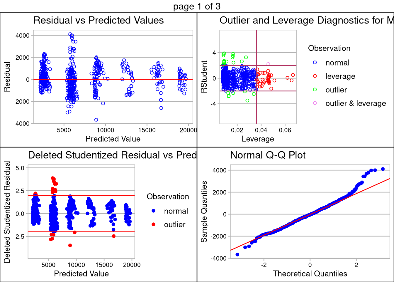
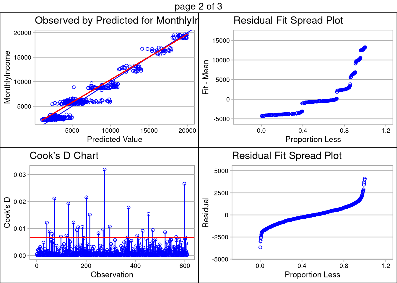
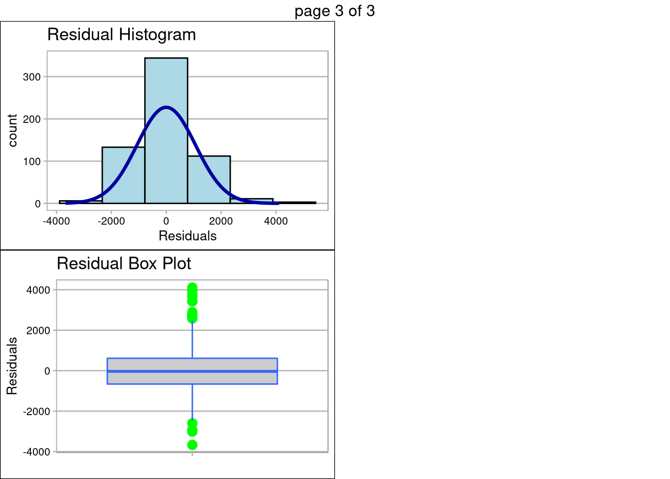
Multiple linear regression is sensitive to co-linearity of features. Using the correlation matrix above, we determined the simplest model uses only JobLevel, TotalWorkingYears, and JobRole for prediction. The TotalWorkingYears and JobLevel features are both highly significant (p-values <.0001) and have a large impact on the estimated salary regression line.
The plot below the prediction summary validates the assumptions of linear regression are met. The data appears normally distributed (as seen in the QQ Plot), the features are linearly correlated, there are no extreme outliers with high influence, and standard deviation among the plots is equal less a few outliers. Transformation of the data did not help with the inequality of variance, so caution should be used when making inference on monthly salary, especially n the ~$5,000/month range.
set.seed(7)
  trainIndices = sample(1:dim(rdata)[1],round(splitPerc * dim(rdata)[1]))
  train = data[trainIndices,]
  test = data[-trainIndices,]
salFit <- lm(MonthlyIncome ~
               JobLevel +
               TotalWorkingYears +
               JobRole
             ,data=train)
summary(salFit)
##
## Call:
## lm(formula = MonthlyIncome ~ JobLevel + TotalWorkingYears + JobRole,
## data = train)
##
## Residuals:
## Min 1Q Median 3Q Max
## -3669.2 -661.0 -34.7 613.6 4106.0
##
## Coefficients:
## Estimate Std. Error t value Pr(>|t|)
## (Intercept) -25.671 260.270 -0.099 0.92146
## JobLevel 2762.115 98.253 28.112 < 2e-16 ***
## TotalWorkingYears 49.968 9.242 5.407 9.29e-08 ***
## JobRoleHuman Resources -409.005 297.717 -1.374 0.17002
## JobRoleLaboratory Technician -580.693 217.614 -2.668 0.00783 **
## JobRoleManager 4097.501 277.600 14.760 < 2e-16 ***
## JobRoleManufacturing Director 116.621 206.533 0.565 0.57252
## JobRoleResearch Director 4059.775 264.269 15.362 < 2e-16 ***
## JobRoleResearch Scientist -357.981 216.054 -1.657 0.09806 .
## JobRoleSales Executive -50.411 186.455 -0.270 0.78697
## JobRoleSales Representative -494.479 263.957 -1.873 0.06151 .
## ---
## Signif. codes: 0 '***' 0.001 '**' 0.01 '*' 0.05 '.' 0.1 ' ' 1
##
## Residual standard error: 1077 on 598 degrees of freedom
## Multiple R-squared: 0.9483, Adjusted R-squared: 0.9474
## F-statistic: 1096 on 10 and 598 DF, p-value: < 2.2e-16salPrd <- predict(salFit, interval="predict",newdata = test)
RMSE <- sqrt(mean((salPrd[,1] - test$MonthlyIncome)^2))
RMSE## [1] 1033.745olsrr::ols_plot_diagnostics(salFit)